2D truncated unimodal example

This example shows how to use lightkde.kde_2d with and without a limit and how it compares to scipy.stats.gaussian_kde for a truncated unimodal bivariate distribution.

Import packages

import matplotlib.pyplot as plt
import numpy as np
from scipy.stats import gaussian_kde, multivariate_normal

from lightkde import kde_2d

Generate synthetic data from a univariate normal distribution and truncate it:

np.random.seed(42)
sample = multivariate_normal.rvs(mean=[0, 0], size=8000)
sample = sample[sample[:, 0] > 0]

Estimate kernel density using lightkde:

density_mx_without_x_min, x_mx_without_x_min, y_mx_without_x_min = kde_2d(
    sample_mx=sample
)
density_mx_with_x_min, x_mx_with_x_min, y_mx_with_x_min = kde_2d(
    sample_mx=sample, xy_min=[0, -5]
)

Estimate kernel density using scipy:

gkde = gaussian_kde(dataset=sample.T)
xy_mx = np.hstack(
    (x_mx_without_x_min.reshape(-1, 1), y_mx_without_x_min.reshape(-1, 1))
)
scipy_density_mx = gkde.evaluate(xy_mx.T).reshape(x_mx_without_x_min.shape)

Plot the data against the kernel density estimates:

bins = (30, 30)
data_density_mx, xedges, yedges = np.histogram2d(
    sample[:, 0], sample[:, 1], bins=bins, density=True
)
z_min = 0
z_max = np.max(data_density_mx)
x_min, x_max = -0.5, max(xedges)
y_min, y_max = min(yedges), max(yedges)

# plot
cmap = "afmhot_r"
fig, ((ax1, ax2), (ax3, ax4)) = plt.subplots(
    2, 2, figsize=(8, 7), sharex="all", sharey="all"
)

# data
h = ax1.hist2d(
    sample[:, 0],
    sample[:, 1],
    bins=bins,
    density=True,
    vmin=z_min,
    vmax=z_max,
    cmap=cmap,
)[-1]
ax1.set_title("data")

# scipy
ax2.contourf(
    x_mx_without_x_min,
    y_mx_without_x_min,
    scipy_density_mx,
    levels=50,
    vmin=z_min,
    vmax=z_max,
    cmap=cmap,
)
ax2.set_xlim(x_min, x_max)
ax3.set_ylim(y_min, y_max)
ax2.set_title("scipy.stats.gaussian_kde")

# lightkde
ax3.contourf(
    x_mx_with_x_min,
    y_mx_with_x_min,
    density_mx_with_x_min,
    levels=50,
    vmin=z_min,
    vmax=z_max,
    cmap=cmap,
)
ax3.set_title("lightkde; with x_min=0")

ax4.contourf(
    x_mx_without_x_min,
    y_mx_without_x_min,
    density_mx_without_x_min,
    levels=50,
    vmin=z_min,
    vmax=z_max,
    cmap=cmap,
)
ax4.set_title("lightkde; without x_min")

fig.subplots_adjust(right=0.80)
cbar_ax = fig.add_axes([0.85, 0.15, 0.05, 0.7], aspect=50)
fig.colorbar(h, cax=cbar_ax, label="density")
plt.show()

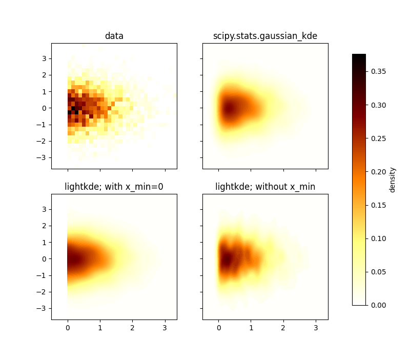
When x_min=0 is used, lightkde approximates well the histogram of the data.