1D truncated unimodal example

This example shows how to use lightkde.kde_1d with and without a limit and how it compares to scipy.stats.gaussian_kde for a truncated unimodal distribution.

Import packages

import matplotlib.pyplot as plt
import numpy as np
from scipy.stats import gaussian_kde, norm

from lightkde import kde_1d

Generate synthetic data from a univariate normal distribution and truncate it:

np.random.seed(42)
sample = norm.rvs(size=2_000)
sample = sample[sample > 0]

Estimate kernel density using lightkde:

density_vec_without_x_min, x_vec_without_x_min = kde_1d(sample_vec=sample)
density_vec_with_x_min, x_vec_with_x_min = kde_1d(sample_vec=sample, x_min=0)

Estimate kernel density using scipy:

gkde = gaussian_kde(dataset=sample)
scipy_density_vec = gkde.evaluate(x_vec_without_x_min)

Plot the data against the kernel density estimates:

fig, ax = plt.subplots(figsize=(6, 4))
ax.plot(x_vec_with_x_min, density_vec_with_x_min, "--r", label="lightkde; with x_min=0")
ax.plot(
    x_vec_without_x_min,
    density_vec_without_x_min,
    ":r",
    label="lightkde; without x_min",
)
ax.plot(
    x_vec_without_x_min, scipy_density_vec, zorder=1, label="scipy.stats.gaussian_kde"
)
ax.hist(sample, bins=30, density=True, alpha=0.5, label="data")
ax.legend()
plt.show()

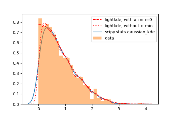
When x_min=0 is used, lightkde approximates well the histogram of the data. Without this option it behaves similarly to the scipy method, both extend to a region without data.